Marketing Mix Modeling (MMM) Explained

Editor's Note: Don’t miss our upcoming webinar: Beyond Multi-Touch: The Resurgence Of Marketing Mix Modeling happening October 13. View the event details and register to attend.
What is MMM (Marketing Mix Modeling)?
Renowned physicist Neils Bohr once famously said, “Prediction is very difficult, especially if it’s about the future.” While this quote may have been a bit tongue-in-cheek, it also touches on a very valuable topic for data scientists and marketers alike: predicting what marketing budget will give you the best return on investment (ROI). In this article, we will demonstrate how Marketing Mix Modeling (MMM), a modeling process that can be used to explain your historical sales data using historical marketing budgets and other non-marketing factors, can be utilized to measure the effectiveness of your marketing efforts and allow you to optimize future marketing budgets.
Marketing Mix Modeling may sound like an intimidating and complicated process. But the logic behind it is actually quite simple. Through MMM, we are simply trying to answer the question, “What fraction of my sales are due to marketing?” Our approach to doing this is to develop a model that solves the following equation:
Sales = Sales from Marketing + Sales from Non-Marketing
In this article, we will greatly expand on what “Sales from Marketing” and “Sales from Non-Marketing” include, and how we estimate them. But it is important to remember that Marketing Mix Modeling is simply a model that tries to build an equation which estimates what fraction of your sales are due to different marketing-related efforts and non-marketing-related factors that may affect your sales.
We will construct an MMM using a fictitious bike sales dataset consisting of five years of weekly sales and marketing spends across 7 different channels (Branded Search, Facebook, Non-Branded Search, Out of Home (OOH), Print, Radio, and TV Spends). From this model, we will be able to estimate the ROI of each individual marketing channel. A visual of both our sales data and historical marketing spends is shown below.
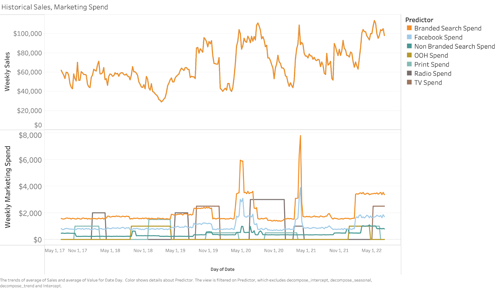
Note to readers: 5 years’ worth of sales and media spend is not necessary for this type of analysis. (Typically we advocate for at least two years so that we have two complete seasonal cycles.) MMMs are able to be built at increasingly detailed levels of granularity for both sales and marketing. An example of this might be that you have sales across different geographic regions or lines of business, or that you are able to break out your marketing budgets by different channels (e.g. paid search in Google vs. paid search in Bing, TV spend on Channel A vs. Channel B). Simply put, the more detailed your data is, the more detailed your model can be.
An MMM’s primary objective is to model our sales data using a combination of marketing and non-marketing data. Answering a question like “What is the ROI of Branded Search, Facebook, Non-Branded Search, Out of Home (OOH), Print, Radio, and TV Spends?” or “What is the effect on sales of a branded paid search campaign in January compared to advertising on YouTube in July?” is possible through Marketing Mix Modeling! We do this by asking the question, “What fraction of my sales can I explain WITHOUT marketing spends?” and then ask “What fraction of sales can I ONLY explain WITH marketing spends?” Allow us to explain further in the next section.
Principles of MMM
Using a technique known as time series decomposition, we first attempt to explain as much of our sales data as possible WITHOUT modeling marketing spends. Time series decomposition is an attempt to explain our sales dataset by breaking it into different components. Typically a time series (BTW, don’t be intimidated by this phrase–it is just a value (sales) that changes over time) over a long period (at least two years) of time can be explained through some combination (either by adding or multiplying) a trend component, a seasonal component, and a remainder component. The trend component is akin to a slowly changing baseline (for example, long term increase in demand for bluetooth headphones compared to declining demand for wire headphones). The seasonal component is the fraction of your time series explained by routine seasonal fluctuations (think change in retail bicycle demand in June compared to January). The remainder component is simply what is left that cannot be explained with trend or seasonality. The formulas for additive and multiplicative decomposition are shown below.
Additive Decomposition
Time Series = trend + seasonal + remainder
Multiplicative Decomposition
Time Series = trend x seasonal x remainder
For demonstration purposes, we will only decompose our dataset with the first approach (additive). But in some instances a multiplicative decomposition may be the right approach for you. Our initial weekly sales data / time series is shown below.
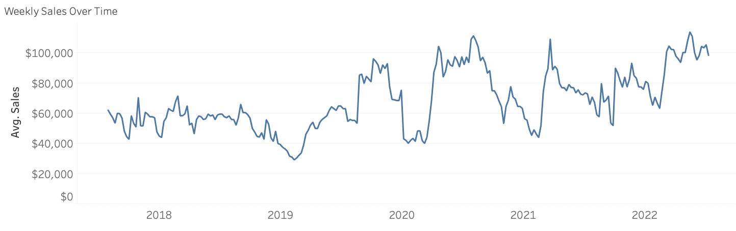
After applying time series decomposition to the dataset above, we are left with the following three components below.
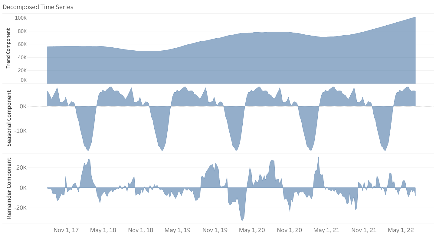
Notice how if you add these three components together, the result is equal to our initial weekly sales.
Our focus now is on the “Remainder” component. This is the component of our time series that is unexplainable by trend or seasonality. Our next step will be to try and explain this component in our model through a multivariate regression technique. Again, do not be intimidated by “multivariate regression.” This just means we are trying to explain what predictors (marketing spends) increase or decrease our sales and by how much. Multivariate regression analysis can either be analytical (one possible solution) or statistical (multiple simulated solutions).
In this analysis, we attempt to measure the effects of marketing on our remainder component through an increasingly popular statistical approach as opposed to a purely analytical solution. A statistical approach to regression attempts to explain our model by evaluating many different simulated solutions to a regression problem and estimating the most likely solution based on the range of possible solutions, whereas an analytical solution arrives at only one possible solution. A more in-depth comparison of these approaches can be found here. At Bounteous, we understand that when it comes to modeling people’s purchasing behavior, there are many factors at play, the effects from marketing are complex, and we believe a model that evaluates many different solutions is the best approach.
All of this aside, for the purposes of this article, it is important to remember at the heart of our analysis, we are now attempting to solve this equation:
Sales From Marketing =Sales From Paid Search + Sales From Facebook + Sales From TV ...
By allowing our model to iterate through thousands of possible solutions, we are able to statistically estimate the most likely effects of our different marketing spends! Our final model, of course, aims to “predict” sales. The more accurate our model is, the more faith we should have in our model components (ROI of marketing spends). So what does this model look like? In its simplest form, our model should be judged by the actual sales (blue line) compared to our model predicted sales (orange line) shown in the table below.
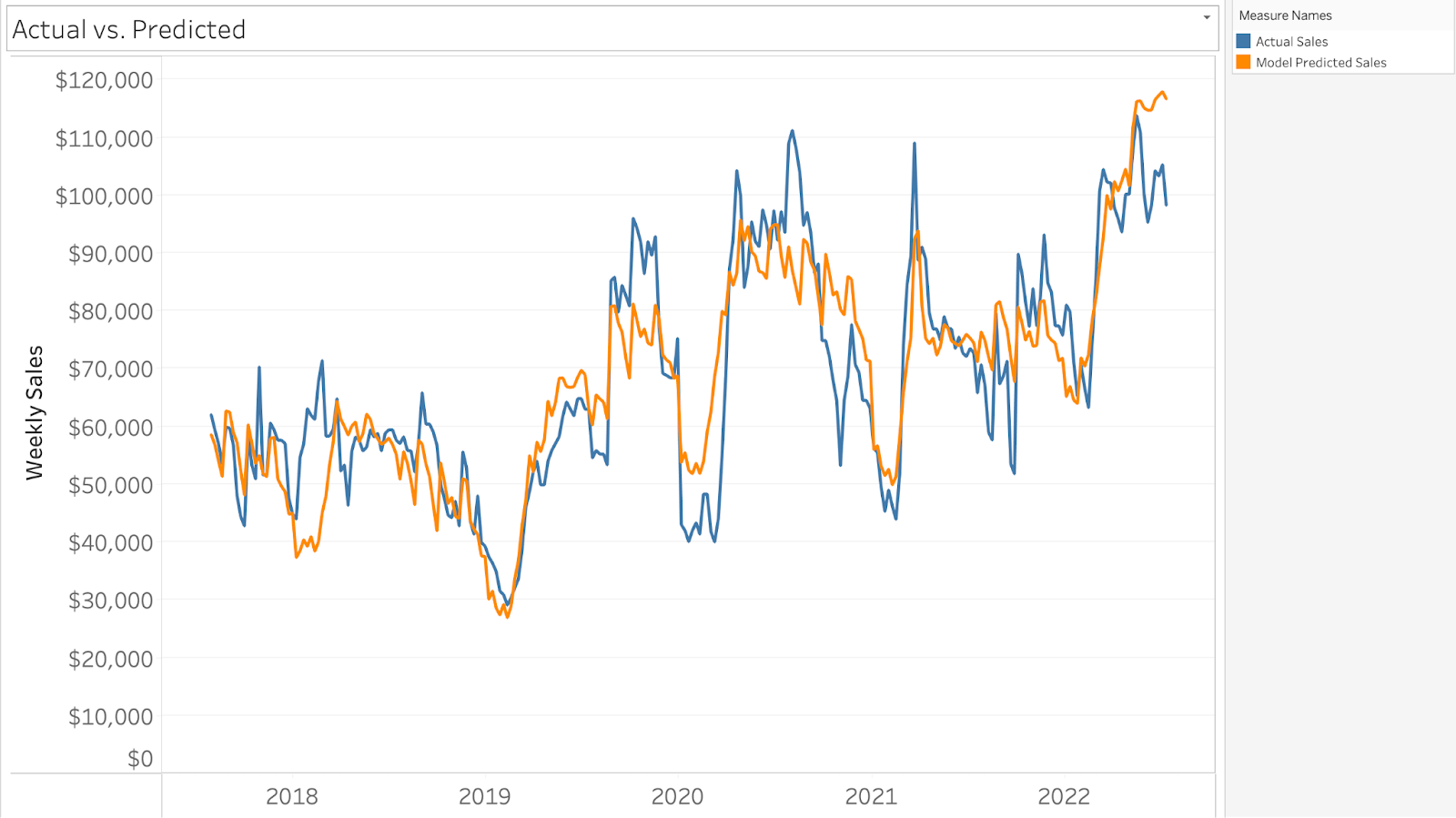
Some common ways to evaluate the quality of a regression model are to compare the actual vs. predicted values for a training and test set. We can do this by way of R Squared (R^2), Mean Absolute Error (MAE), Mean Absolute Percentage Error (MAPE), Root Mean Square Error (RMSE), and Normalized Root Mean Square Error (NRMSE) calculations.
| Model Evaluator | Value | Acceptable Value |
|---|---|---|
| R^2 | .87 | > .7 |
| MAE | $7,402 | N/A |
| MAPE | 11.4% | < 10% good, 10-25% acceptabl |
| RMSE | $9,677 | N/A |
| NRMSE | .11 | < .1 good, .1 - .25 acceptable |
The evaluations shown above are from in-sample comparisons only. In a more scrupulous evaluation, the same calculations would be applied to both a random holdout (random points in dataset) or last n data points (for example, holding out the last n months’ worth of data) to evaluate your model’s ability to predict future sales. A more in-depth analysis would also evaluate actual versus predicted ‘sales due to marketing.’
Now that we have established that our model has an acceptable level of accuracy, an obvious next question is “How much of our sales are due to marketing?” The visual below provides this information.
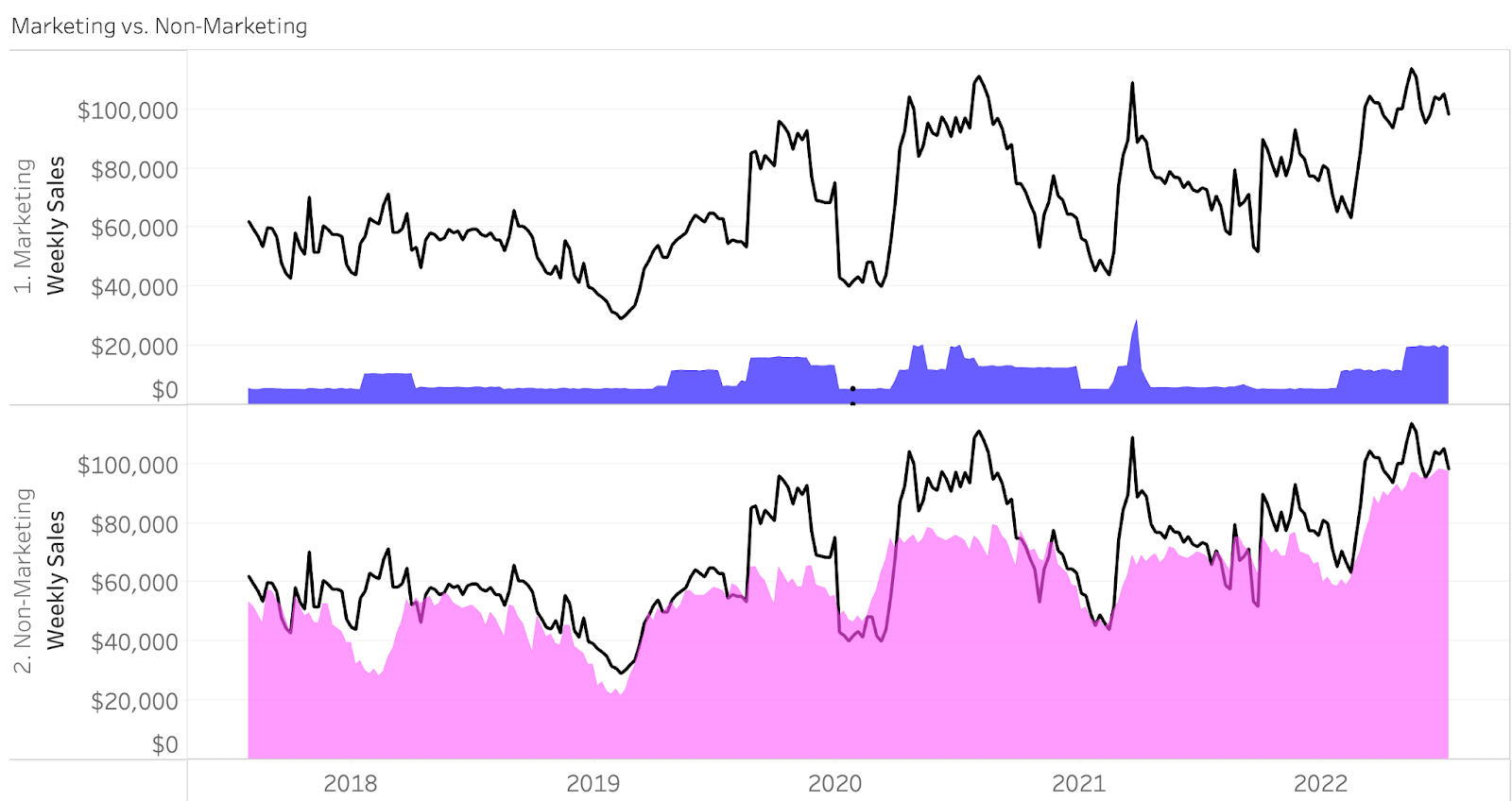
The black line in this plot is our actual sales, and the shaded areas represent model predicted sales due to Marketing and Non-Marketing. Another way to contextualize this would be what percentage of my total sales are due to marketing over time? (visualized below)
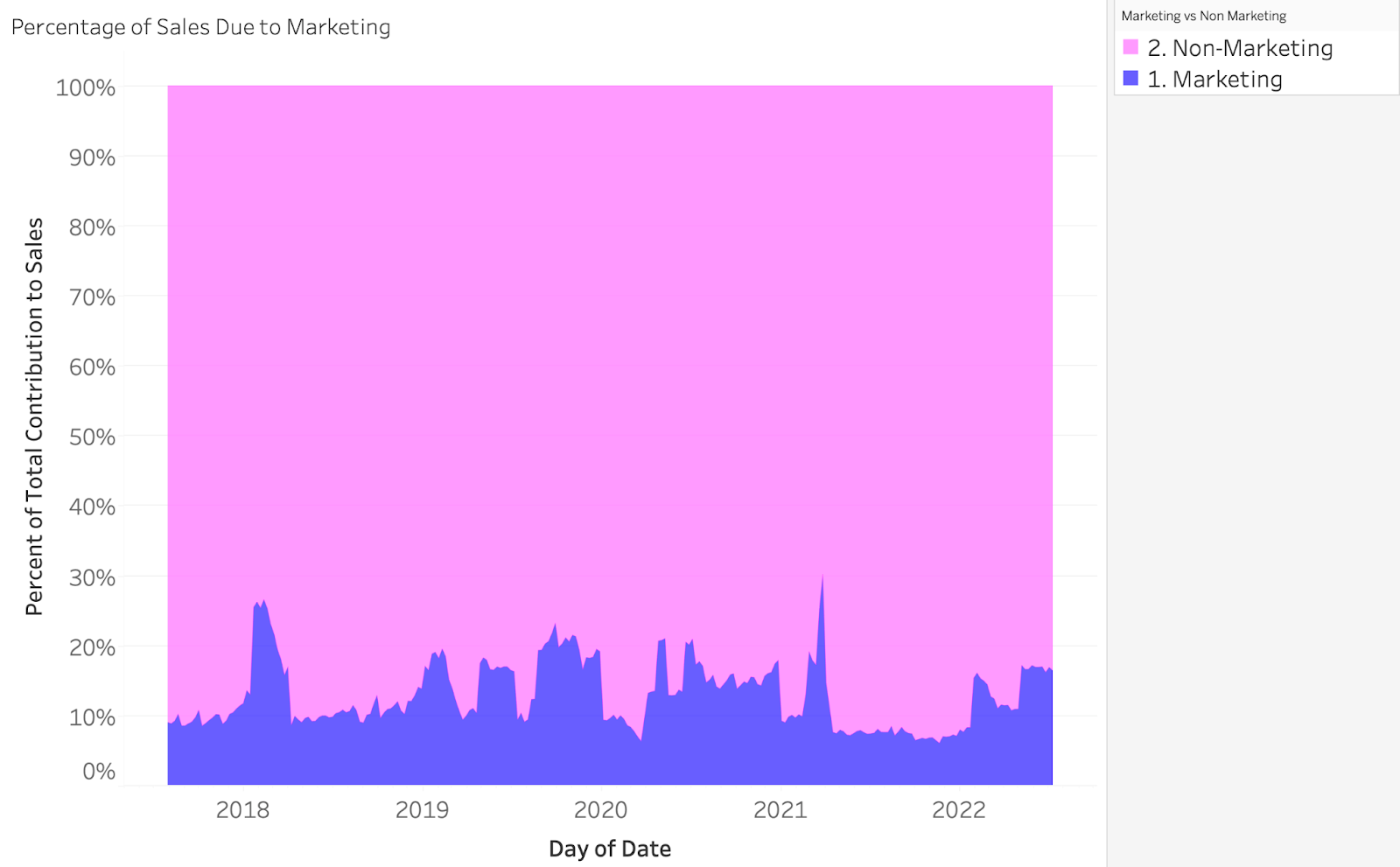
Our takeaway from this is that sales due to marketing, on average, represents around 10% of our total sales. In some extreme cases we estimate the effects of marketing to be upwards of 20-30%. This can be directly traced back to significant increases in our historical marketing budgets. In the cases of both Marketing and Non-Marketing sales, we can dive much deeper into the composition of our model (below).
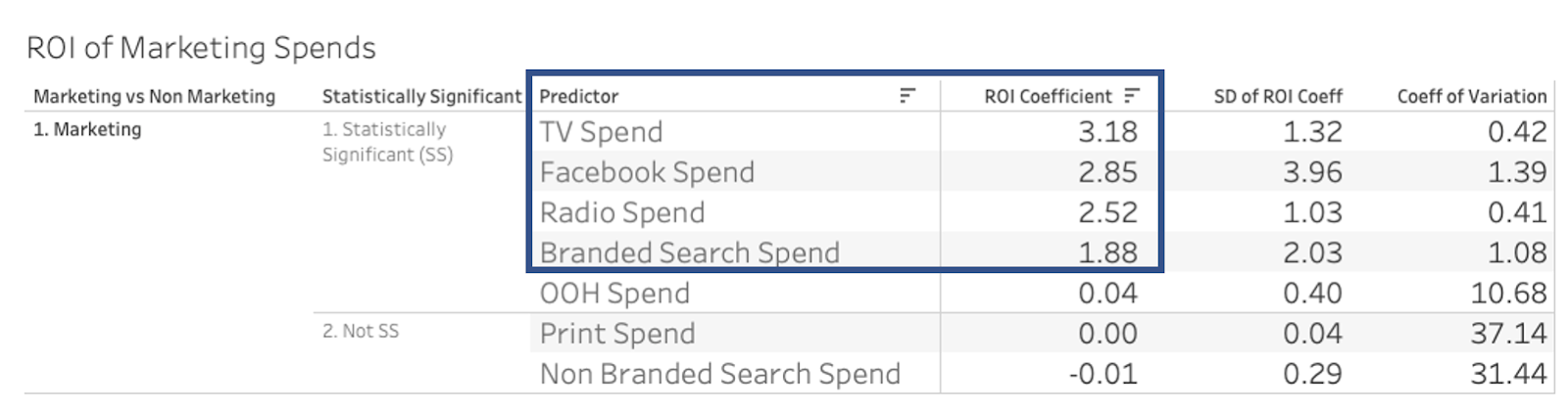
The table below shows us our estimated ROI from the different marketing spends over time. From this table we can see that TV Spend, Facebook Spend, Radio Spend, and Branded Search Spend are estimated to have positive ROI (ROI > 1 is considered to be positive, implying that for every dollar you spend you get > $1 in return).
We define a statistically significant ROI coefficient based on the absolute value of the Standard Deviation / Mean. This is referred to as the Coefficient of Variation. Typically a Coefficient of Variation < 30 is considered to be statistically significant. A literal interpretation from this table is “for every dollar you spend in TV advertising, you are getting $3.18 in sales; for every dollar you spend in Facebook advertising, you are getting $2.85 in sales.” Our model also shows that based on our definition of ROI positive and statistically significant, 4 of 7 marketing channels are both positive and statistically significant.
The ROI coefficients shown in the table are what we use to reconstruct our initial formula. If we recall, previously we stated that:
Sales From Marketing = Sales From Facebook + Sales From Branded Paid Search + .....
A more detailed version of this equation would read:
Sales Due to Marketing = ROI Facebook x FB Spend + ROI Branded Search x BS Spend + ...
With these equations in mind, we can now explain both our sales due to non-marketing factors (seasonality, trend, intercept) and our estimated sales due to marketing (Facebook, Branded Search, TV etc). This visual is below:
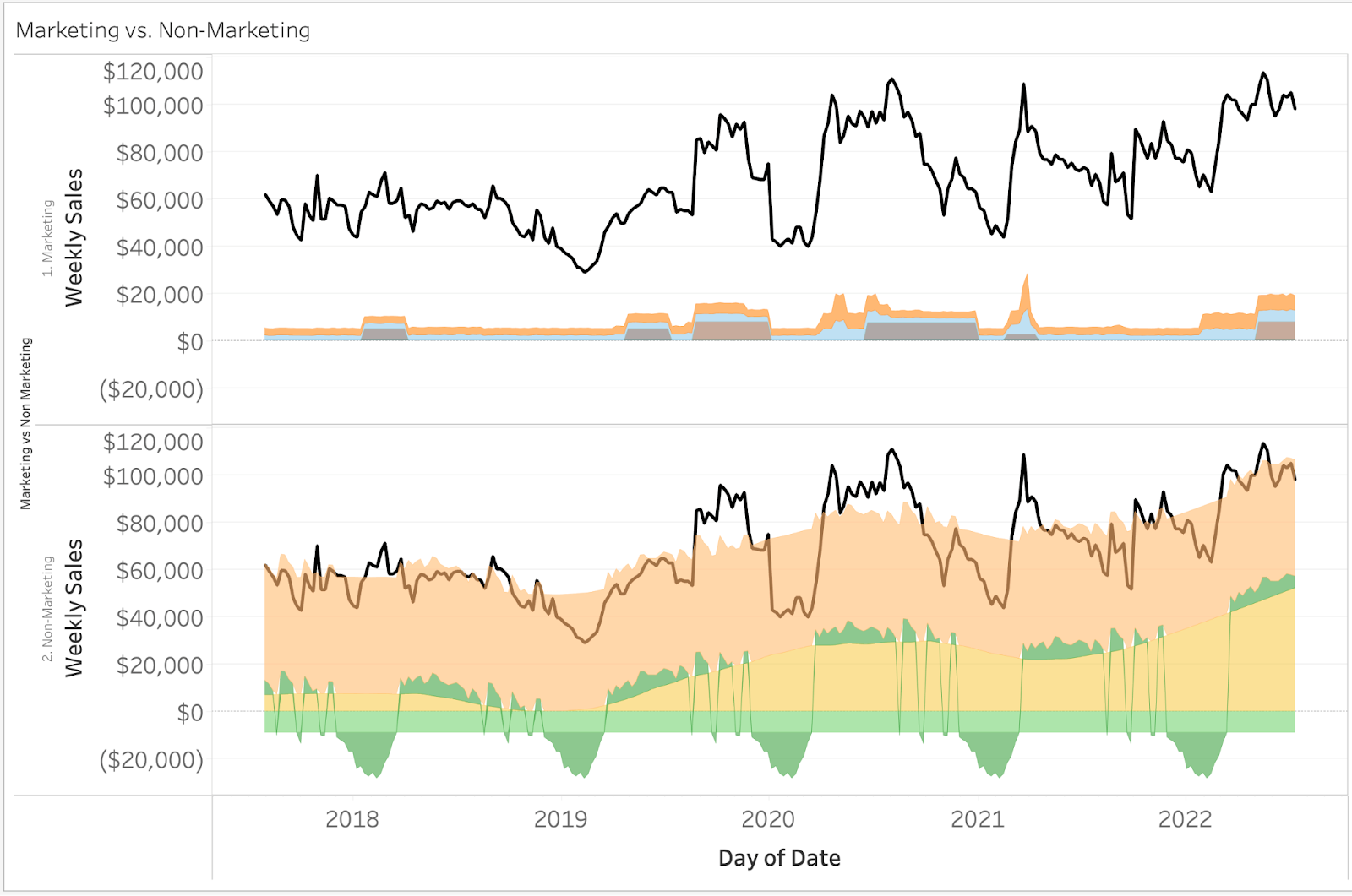
The top chart shows our estimated sales due to marketing. Each color represents sales due to a different marketing tactic. Similarly, the bottom chart shows sales to do non-marketing where the different colors represent different trends and seasonalities in our dataset. A more rigorous analysis would aim to trace these seasonalities back to factors that are likely to affect your line of business (macroeconomic conditions, changes in distribution, weather etc). Do you know how much your sales increase/decrease when the average daily temperature increases or when the price of a barrel of oil decreases? Media Mix Modeling has the ability to uncover this as well! In the next visual, we will dive directly into our sales due to marketing. As a reference, we can even compare the estimated sales due to marketing with our actual marketing spends.
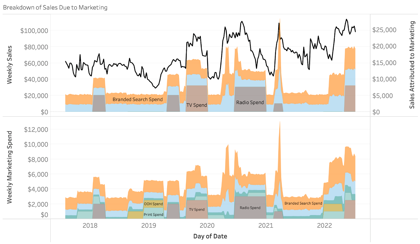
The visual above reveals many details of our analysis, including:
- Weekly Sales (black line top chart)
- Sales Attributed to Marketing (area chart top)
- Weekly Marketing Spends (area chart bottom right)
A quick look at our visual and we can see that weekly marketing spends range between $2k - $12k and are netting estimated returns in sales between $5k - $25k. As a reference, our weekly sales are between $28k and $111k. Notice how during certain timeframes a surge in spending for a particular channel lines up with a surge in sales. An example of this is seen specifically for branded search during the timeframe February, 16 2020 - April, 17 2022 as shown below.
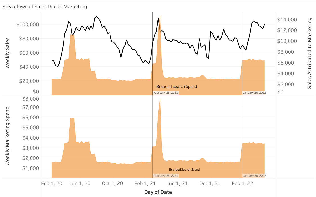
If we look closely, we can see that our increases in Branded Search Spend on February 28, 2021 and January, 30, 2022 line up with increases in sales. These types of patterns are how our model is able to estimate the ROI of our different marketing spends, and a good example of why constant testing and fluctuations in spend should be an essential part of your marketing strategy!
Activating on MMM
From this analysis, we are able to learn that TV Spend, Facebook Spend, Radio Spend, and Branded Search Spend are positive and statistically significant drivers of sales and OOH, Print Spend, and Non-Branded Spend are not. A natural takeaway from this would be to reduce spending for Print and Non-Branded and increase spending for TV, Facebook, Radio, and Branded. Perhaps, at this point you are thinking, “I should spend all of my money on TV Spend.” It is important to remember that this analysis is called Media MIX Modeling because we are modeling the mix of media spending. The results of this analysis do not neccesarily mean that we would advocate for abandoning spend in channels where we were not able to measure statistically significant positive ROI, nor do they mean we would advocate for going “all in '' on our most effective channel. Instead, we would advocate for strategic adjustments to budgets based on the findings of our model and continued testing of the resulting effects on sales.
A more comprehensive analysis might look into other less direct relationships between sales and our marketing tactics. Perhaps you think that your cumulative increases in marketing spend over several years is slowly increasing your sales, so can a model prove this? Another question you might have is does a relationship between the combined spend between branded paid search and TV spend two weeks prior exist? Or is there a relationship between non-branded paid search spend from three weeks ago and branded search spend from a week ago and my sales this week? These types of questions and more are all able to be answered through MMM!