How To Bulk Redirect Complicated URLs
You have thousands of product images stored across many different directories on your website. In an effort to keep things more organized you decide to consolidate those images to one directory on your website, leaving you with the task of creating a best match redirect map for the old images to their new directory. The only similarity between the new and old URLs is the product name. Below I’ll show you how to use regular expression and Excel to make a best match redirect map for complex URLs, leaving you more time to kick back and chill.
You can follow along with this example spreadsheet.
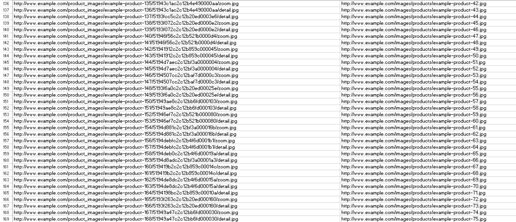
Step 1: Compile a list of all 404 URLs and all possible live (202) URLs. Moving forward I will assume you have already done this. Below is a snapshot of my example’s URLs. The left column contains the live URLs, and the right column contains the 404 URLs.

Step2: Deconstruct the URLs using regular expressions so that each part of the URL is separated by tabs (instead of backslashes).
The expression looks like this:
Find: ^http://www.example.com/(.+)/(.+)/(.+).(.+)$
Replace with: http://www.example.comt$1t$2t$3t$4
The regular expression above captures the areas between each backslash and then places them in-between tab strokes instead. Doing this creates a tab-delimited file which will allow you to do a quick copy/paste into excel. Excel recognizes the tab spaces when you do this, and places each section of the URL into its own column.
This is what each URL should look like before and after:
Before: http://www.example.com/images/extraLarge/example-product-1.jpg
After: http://www.example.com images extraLarge example-product-1 jpg
If you aren’t familiar with regular expressions “.” looks for any single character (i.e. a-z, 0-9, and spaces), and the “+” tells the text editor to look for 1 or more of any character. When these two are placed inside parenthesis it groups them.
^http://www.example.com/ – The carrot denotes the beginning of the strings of characters you want to match, and the rest matches an exact string of characters.
1st (.+) – matches everything in-between the backslash before and after it. The second (.+) operates the same way.
3rd (.+) – matches the product image. At this point, we could match the entire image name – examples-product-1.jpg. But because our new url structure is more complicated than the original, we need to break out the file extension from the file name.
. – escapes the period making it a normal character, not a regular expression character. The escaped period now acts like the backlash and allows us to replace it with a tab break.
4th (.+) – Captures the file extension (jpg, png, gif, etc.).
$ – Tells the text editor that it has reached the end of the string you’re looking for.
Step 3: Use VLOOKUP and CONCATENATE to find and match URLs.
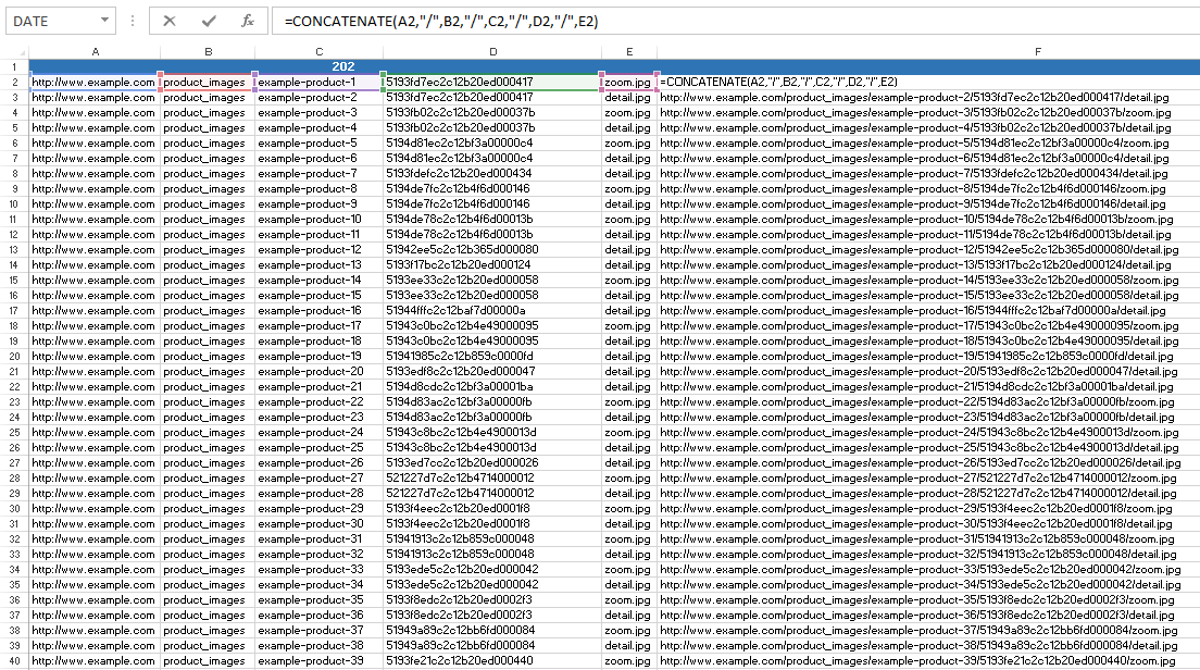
Once you have created the tab-delimited files for your list of 404 and 202 URLs, it’s time to plug them into Excel and match them. In this example the 202 URLs take up 5 columns – A through E – so in column F we will recompile the URL and use it as a helper column during our VLOOKUP.

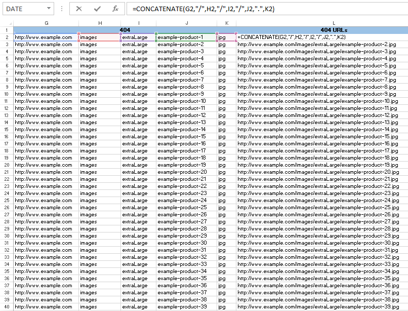
You will need to do the same with the 404 URLs.

As you can see the concatenate function is referencing cells that contain portions of the URL and is inserting backslashes (and a period) back into the URLs’ structure.
Once you have that it’s time to make the matches with VLOOKUP. Using the two columns that contain unique product information – column C and column J – use VLOOKUP to find each 404 product (column J) within an array of all new products (column C), and have it return our concatenated helper column – column F. The function will look like this:
=VLOOKUP(J2,$C$2:$F$6857,4,0)

The VLOOKUP function is working like so:
J2 – is the value you want to look up. Within the function, it's labeled ‘lookup_value’.
$C$2:$F$6857 – defines the array within which your lookup value exists – column C – and includes the value you would like to return – column F. Within the function this is labeled ‘table_array’. VLOOKUP always looks through the first column in this array to match your lookup_value.
4 – denotes the column within the array that you would like to return. Because we would like to return the complete URL related to the match, we return the concatenated column, column F. Within the function this is called ‘col_index_num’.
0 – zero (or FALSE) tells VLOOKUP we want an exact match. Within the function, it’s called ‘range_lookup’
Copy and paste that VLOOKUP function to the bottom of your 404 list, copy columns L (404 URL) and column M – the matching 202 URL – then paste them as data into a new spreadsheet. You now have a 404 redirect map for thousands of complex URLs.


