How to Use Time Elements From Google Analytics in Excel

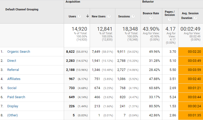
If you’ve ever tried downloading the All Pages or Channels reports from Google Analytics as an Excel spreadsheet, you may have noticed that your time metrics look a little different. Instead of looking like a time element, the Avg. Time on Page and Avg. Session Duration metrics are formatted as numbers showing the number of seconds, rather than the hh:mm:ss format used in Google Analytics. This can be especially frustrating for anyone who downloads reports into Excel regularly, or shares these Excel spreadsheets through scheduled emails.
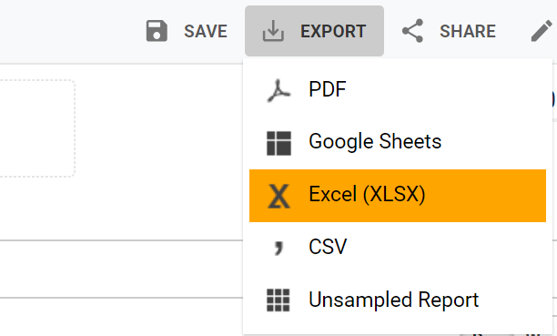
Note - this happens when downloading reports from the Google Analytics interface using the Excel (XLSX) option, or accessing data through the API, but usually not when downloading a CSV or using the Google Sheets options.
So why does this happen, and how can we make it look like a time element again?
Excel Prefers Number Formats
By default, Excel uses the General format, which means the numbers appear just as you type them - no commas, rounding, or other special formatting. This is why time metric formats are automatically shown as the number of seconds spent on the page or session. The General format actually makes it easy to compare different pages or sites, see how things are increasing or decreasing, and perform calculations and averages. If you need to do any of that, you should keep the General format.
Numbers don’t look like “Time”
Unfortunately, the General format isn’t great for graphs, charts, or tables. It’s hard for us to look at numbers and convert that to time — especially when we want a quick visual. If we’re talking about making things look pretty or easy to understand, we can do also do that in Excel, but keep in mind it might make it hard to do calculations, averages, etc.
Time in Excel is Relative to Days
If you want to do anything in Excel involving dates, the base unit is one day. Excel stores dates as serial numbers, beginning with January 1, 1900, as serial number 1. The serial number for January 1, 2019, is 43,466 because the date is 43,465 days after January 1, 1900. This way, you can take a date in Excel, and add the number 1 to it, and it will show you tomorrow’s date. So, when we’re looking to show something like minutes and seconds, we need to convert it to fit Excel’s format, which means part of a day.
Solution One: Text Value Pre-Formatted
The quickest and easiest way to make your time metrics look right for your report would be to convert it into text that looks correct. Again, this makes it hard to do anything with comparisons or calculations, even greater than or less than.
Let’s do an example together.
Step 1
When you download your All Pages report to Excel, Avg. Time on Page will fall in column D. You will need to insert a new column between D & E — labeled E1, and E2.
Step 2
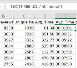
In E1, copy over your label ‘Avg. Time on Page’. In E2, add the formula, =TEXT(TIME(,,D2),"hh:mm:ss". The TIME function converts your time elapsed in seconds to a portion of a day. The TEXT function then allows us to reformat this number to match the Google Analytics format.
Once E1 and E2 are populated with the correct information, hit enter. Then, copy and paste that formula to the entire column, or ‘drag down’ the formula. You can do this by clicking on E2, then clicking the small black box in the bottom right corner of the cell, click and hold, and drag that to the bottom of the cell. Or simply double click the box to autofill.
Solution Two – Date with the Correct Number Format
This method is a little bit more robust. You can do comparisons, calculations, etc., but it requires some additional understanding. In every cell, you have two things that we care about - the “CELL VALUE” and the “NUMBER FORMAT” of the cell. You’ve likely encountered this is you’ve changed numbers into currency, etc. The number in the cell stays the same, but it looks a little different.
Let's walk through solution two.
Step 1
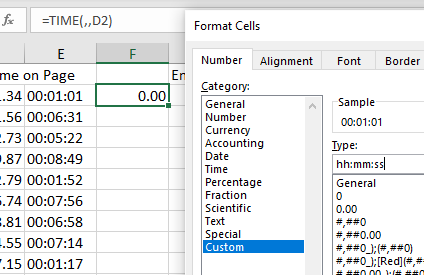
First, insert a new column between D & E — again, labeled E1 and E2. In E1, copy over your label ‘Avg. Time on Page’. In E2, add the formula =TIME(,,D2).
Step 2
Right-click on the cell and choose “Format Cell” (or Cmd+1 for Mac users, Ctrl+1 for PC). Under the Number tab, click on the Custom option and paste in the number format, hh:mm:ss. Once this is pasted, hit enter. Then copy and paste the formula into the entire column, or ‘drag down’ the formula.
In Summary
Spreadsheet tools like Excel and Google Sheets are great tools for creating reports and analyzing data. Understanding the underlying methods for storing and displaying data are helpful when tackling issues like this one. Use these methods of formatting to make Excel work best for your Google Analytics data!
